Plot 2

#!/usr/bin/env python3
"""
@author: Quentin Rodier
Creation : 07/01/2021

Last modifications
"""
import matplotlib as mpl
mpl.use('Agg')
from read_MNHfile import read_netcdf
from Panel_Plot import PanelPlot
from misc_functions import mean_operator, convert_date
import cartopy.crs as ccrs
import numpy as np
import os
import cartopy.io.shapereader as shpreader
import matplotlib.patches as mpatches
os.system('rm -f tempgraph*')
#
#  User's parameter / Namelist
#
path=""

LnameFiles = ['AZF02.1.CEN4T.001.nc', 'AZF02.1.CEN4T.002.nc', 'AZF02.1.CEN4T.003.nc',
              'AZF02.1.CEN4T.004.nc', 'AZF02.1.CEN4T.005.nc', 'AZF02.1.CEN4T.007.nc',
              'AZF02.2.CEN4T.001.nc', 'AZF02.2.CEN4T.002.nc', 'AZF02.2.CEN4T.003.nc',
              'AZF02.2.CEN4T.004.nc', 'AZF02.2.CEN4T.005.nc', 'AZF02.2.CEN4T.007.nc',
              'AZF02.1.CEN4T.000.nc']
LG_AVION='/Flyers/Aircrafts/AVION/'
LG_AVIONT='/Flyers/Aircrafts/AVION/Point/'
LG_AVIONZT='/Flyers/Aircrafts/AVION/Vertical_profile/'

Dvar_input = {
'f1':['SVT001','SVT002','ATC001','ATC002','UT','VT','latitude','longitude','level'],
'f2':['SVT001','SVT002','ATC001','ATC002','UT','VT','latitude','longitude','level'],
'f3':['SVT001','SVT002','ATC001','ATC002','UT','VT','latitude','longitude','level'],
'f4':['SVT001','SVT002','ATC001','ATC002','UT','VT','latitude','longitude','level'],
'f5':['SVT001','SVT002','ATC001','ATC002','UT','VT','latitude','longitude','level'],
'f6':['SVT001','SVT002','ATC001','ATC002','UT','VT','latitude','longitude','level'],
'f7':['SVT001','SVT002','ATC001','ATC002','UT','VT','latitude','longitude','level','LONOR','LATOR','LAT','LON'],
'f8':['SVT001','SVT002','ATC001','ATC002','UT','VT','latitude','longitude','level'],
'f9':['SVT001','SVT002','ATC001','ATC002','UT','VT','latitude','longitude','level'],
'f10':['SVT001','SVT002','ATC001','ATC002','UT','VT','latitude','longitude','level'],
'f11':['SVT001','SVT002','ATC001','ATC002','UT','VT','latitude','longitude','level'],
'f12':['SVT001','SVT002','ATC001','ATC002','UT','VT','latitude','longitude','level'],
'f13':[(LG_AVION,'time_flyer'),(LG_AVIONT,'ZS'), (LG_AVIONT,'P'), (LG_AVIONT,'LON'),(LG_AVIONT,'MER_WIND'),
       (LG_AVIONT,'ZON_WIND'),(LG_AVIONT,'W'), (LG_AVIONT,'Th'), (LG_AVIONT,'Rv'),(LG_AVIONT,'Tke'),
       (LG_AVIONT,'H_FLUX'),(LG_AVIONT,'LE_FLUX'), (LG_AVIONT,'Tke_Diss'), (LG_AVIONT,'Tsrad')]
}

#  Read the variables in the files
Dvar = {}
Dvar = read_netcdf(LnameFiles, Dvar_input, path=path, removeHALO=True)

################################################################
#########          PANEL 1
###############################################################
Panel = PanelPlot(2,3, [25,14],'Domaine 1 SV 001', titlepad=25, minmaxpad=1.04, timepad=-0.07, colorbarpad=0.03, labelcolorbarpad = 13, colorbaraspect=22)
Lplot = [Dvar['f1']['SVT001'], Dvar['f2']['SVT001'], Dvar['f3']['SVT001'],
         Dvar['f4']['SVT001'], Dvar['f5']['SVT001'], Dvar['f6']['SVT001']]

lon = [Dvar['f1']['longitude']]*len(Lplot)
lat = [Dvar['f1']['latitude']]*len(Lplot)
Ltitle = ['SVT001']*len(Lplot)
Lcbarlabel = ['kg/kg']*len(Lplot)
Lxlab = ['longitude']*len(Lplot)
Lylab = ['latitude']*len(Lplot)
Lminval = [0]*len(Lplot)
Lmaxval = [0.15E-5]*len(Lplot)
Lstep = [0.05E-6]*len(Lplot)
Lstepticks = [0.2E-6]*len(Lplot) 
Lcolormap = ['gist_rainbow_r']*len(Lplot)
Lprojection = [ccrs.PlateCarree()]*len(Lplot)
LaddWhite = [True]*len(Lplot)
Llevel = [0]*len(Lplot)
Ltime = [Dvar['f1']['date'], Dvar['f2']['date'], Dvar['f3']['date'], Dvar['f4']['date'], Dvar['f5']['date'], Dvar['f6']['date']]
Lcbformatlabel=[True]*len(Lplot)
fig = Panel.psectionH(lon=lon, lat=lat, Lvar=Lplot, Lxlab=Lxlab, Lylab=Lylab, Ltitle=Ltitle, Lminval=Lminval, Lmaxval=Lmaxval, 
                                Lstep=Lstep, Lstepticks=Lstepticks, Lcolormap=Lcolormap, Lcbarlabel=Lcbarlabel, 
                                Ltime=Ltime, LaddWhite_cm=LaddWhite, Lproj=Lprojection, Llevel=Llevel, Lcbformatlabel=Lcbformatlabel)

Lplot1 = [ Dvar['f1']['UT'], Dvar['f2']['UT'], Dvar['f3']['UT'], Dvar['f4']['UT'], Dvar['f5']['UT'], Dvar['f6']['UT']]
Lplot2 = [ Dvar['f1']['VT'], Dvar['f2']['VT'], Dvar['f3']['VT'], Dvar['f4']['VT'], Dvar['f5']['VT'], Dvar['f6']['VT']]
Ltitle = ['wind vectors at K=2']*len(Lplot)
Llegendval = [7.5]*len(Lplot)
Lcbarlabel = ['(m/s)']*len(Lplot1)
Larrowstep = [2]*len(Lplot1)
Lwidth = [0.002]*len(Lplot1)
Lcolor = ['black']*len(Lplot1)
Lscale = [100]*len(Lplot1)
fig = Panel.pvector(Lxx=lon, Lyy=lat, Llevel=Llevel, Lvar1=Lplot1, Lvar2=Lplot2, Lxlab=Lxlab, Lylab=Lylab, Ltitle=Ltitle, Lwidth=Lwidth, Larrowstep=Larrowstep,
                      Llegendval=Llegendval, Lcbarlabel=Lcbarlabel, Lproj=Lprojection, Lid_overlap=[0,2,4,6,8,10], ax=fig.axes, Lscale=Lscale)

# Departements francais
departements_shp='departements-20180101.shp'
adm1_shapes = list(shpreader.Reader(departements_shp).geometries())

# Add departements to each axes + scatter point of emission source
loncar, latcar = [1.439,1.5], [43.567, 43.9]
label=['AZF1','AZF2']
for i in range(len(Lplot)):
  fig.axes[i*2].add_geometries(adm1_shapes, ccrs.PlateCarree(),edgecolor='black', facecolor='white', alpha=0.2)
  fig.axes[i*2].scatter(loncar,latcar)
  for lab, txt in enumerate(label):
    fig.axes[i*2].annotate(label[lab], (loncar[lab], latcar[lab]), color='black',size=10, weight="bold")

# Add a Rectangle displaying the domain of the model 2
for i in range(len(Lplot)):
  fig.axes[i*2].add_patch(mpatches.Rectangle(xy=[Dvar['f7']['LONOR'], Dvar['f7']['LATOR']], width=Dvar['f7']['LON'][-1,-1]-Dvar['f7']['LONOR'], height=Dvar['f7']['LAT'][-1,-1]-Dvar['f7']['LATOR'],
   facecolor='blue', alpha=0.15, transform=ccrs.PlateCarree()))

fig.tight_layout()
Panel.save_graph(1,fig)

################################################################
#########          PANEL 2
###############################################################
Panel = PanelPlot(2,3, [25,14],'Domaine 1 SV 002', titlepad=25, minmaxpad=1.04, timepad=-0.07, colorbarpad=0.03, labelcolorbarpad = 13, colorbaraspect=22)
Lplot = [Dvar['f1']['SVT002'], Dvar['f2']['SVT002'], Dvar['f3']['SVT002'],
         Dvar['f4']['SVT002'], Dvar['f5']['SVT002'], Dvar['f6']['SVT002']]

lon = [Dvar['f1']['longitude']]*len(Lplot)
lat = [Dvar['f1']['latitude']]*len(Lplot)
Ltitle = ['SVT001']*len(Lplot)
Lcbarlabel = ['kg/kg']*len(Lplot)
Lminval = [0]*len(Lplot)
Lmaxval = [0.15E-5]*len(Lplot)
Lstep = [0.05E-6]*len(Lplot)
Lstepticks = [0.2E-6]*len(Lplot) 
Lcbformatlabel=[True]*len(Lplot)
fig = Panel.psectionH(lon=lon, lat=lat, Lvar=Lplot, Lxlab=Lxlab, Lylab=Lylab, Ltitle=Ltitle, Lminval=Lminval, Lmaxval=Lmaxval, 
                                Lstep=Lstep, Lstepticks=Lstepticks, Lcolormap=Lcolormap, Lcbarlabel=Lcbarlabel, 
                                Ltime=Ltime, LaddWhite_cm=LaddWhite, Lproj=Lprojection, Llevel=Llevel, Lcbformatlabel=Lcbformatlabel)

fig = Panel.pvector(Lxx=lon, Lyy=lat, Llevel=Llevel, Lvar1=Lplot1, Lvar2=Lplot2, Lxlab=Lxlab, Lylab=Lylab, Ltitle=Ltitle, Lwidth=Lwidth, Larrowstep=Larrowstep,
                      Llegendval=Llegendval, Lcbarlabel=Lcbarlabel, Lproj=Lprojection, Lid_overlap=[0,2,4,6,8,10], ax=fig.axes, Lscale=Lscale)

# Add departements to each axes + scatter point of emission source
for i in range(len(Lplot)):
  fig.axes[i*2].add_geometries(adm1_shapes, ccrs.PlateCarree(),edgecolor='black', facecolor='white', alpha=0.2)
  fig.axes[i*2].scatter(loncar,latcar)
  for lab, txt in enumerate(label):
    fig.axes[i*2].annotate(label[lab], (loncar[lab], latcar[lab]), color='black',size=10, weight="bold")

# Add a Rectangle displaying the domain of the model 2
for i in range(len(Lplot)):
  fig.axes[i*2].add_patch(mpatches.Rectangle(xy=[Dvar['f7']['LONOR'], Dvar['f7']['LATOR']], width=Dvar['f7']['LON'][-1,-1]-Dvar['f7']['LONOR'], height=Dvar['f7']['LAT'][-1,-1]-Dvar['f7']['LATOR'],
   facecolor='blue', alpha=0.15, transform=ccrs.PlateCarree()))

fig.tight_layout()
Panel.save_graph(2,fig)

################################################################
#########          PANEL 3
###############################################################
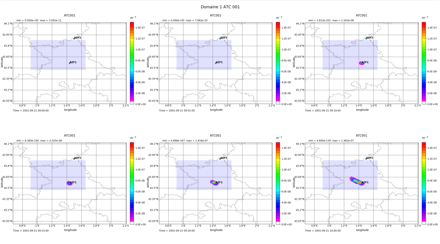
Panel = PanelPlot(2,3, [25,14],'Domaine 1 ATC 001', titlepad=25, minmaxpad=1.04, timepad=-0.07, colorbarpad=0.03, labelcolorbarpad = 13, colorbaraspect=22)
Lplot = [Dvar['f1']['ATC001'], Dvar['f2']['ATC001'], Dvar['f3']['ATC001'],
         Dvar['f4']['ATC001'], Dvar['f5']['ATC001'], Dvar['f6']['ATC001']]

Ltitle = ['ATC001']*len(Lplot)
Lcbarlabel = ['$m^{-3}$']*len(Lplot)
Lminval = [0]*len(Lplot)
Lmaxval = [0.15E-6]*len(Lplot)
Lstep = [0.05E-7]*len(Lplot)
Lstepticks = [0.2E-7]*len(Lplot) 
fig = Panel.psectionH(lon=lon, lat=lat, Lvar=Lplot, Lxlab=Lxlab, Lylab=Lylab, Ltitle=Ltitle, Lminval=Lminval, Lmaxval=Lmaxval, 
                                Lstep=Lstep, Lstepticks=Lstepticks, Lcolormap=Lcolormap, Lcbarlabel=Lcbarlabel, 
                                Ltime=Ltime, LaddWhite_cm=LaddWhite, Lproj=Lprojection, Llevel=Llevel, Lcbformatlabel=Lcbformatlabel)

# Add departements to each axes + scatter point of emission source
for i in range(len(Lplot)):
  fig.axes[i*2].add_geometries(adm1_shapes, ccrs.PlateCarree(),edgecolor='black', facecolor='white', alpha=0.2)
  fig.axes[i*2].scatter(loncar,latcar)
  for lab, txt in enumerate(label):
    fig.axes[i*2].annotate(label[lab], (loncar[lab], latcar[lab]), color='black',size=10, weight="bold")

# Add a Rectangle displaying the domain of the model 2
for i in range(len(Lplot)):
  fig.axes[i*2].add_patch(mpatches.Rectangle(xy=[Dvar['f7']['LONOR'], Dvar['f7']['LATOR']], width=Dvar['f7']['LON'][-1,-1]-Dvar['f7']['LONOR'], height=Dvar['f7']['LAT'][-1,-1]-Dvar['f7']['LATOR'],
   facecolor='blue', alpha=0.15, transform=ccrs.PlateCarree()))

fig.tight_layout()
Panel.save_graph(3,fig)

################################################################
#########          PANEL 4
###############################################################
Panel = PanelPlot(2,3, [25,14],'Domaine 1 ATC 002', titlepad=25, minmaxpad=1.04, timepad=-0.07, colorbarpad=0.03, labelcolorbarpad = 13, colorbaraspect=22)
Lplot = [Dvar['f1']['ATC002'], Dvar['f2']['ATC002'], Dvar['f3']['ATC002'],
         Dvar['f4']['ATC002'], Dvar['f5']['ATC002'], Dvar['f6']['ATC002']]

Ltitle = ['ATC002']*len(Lplot)
Lcbarlabel = ['$m^{-3}$']*len(Lplot)
Lminval = [0]*len(Lplot)
Lmaxval = [0.15E-6]*len(Lplot)
Lstep = [0.05E-7]*len(Lplot)
Lstepticks = [0.2E-7]*len(Lplot) 
fig = Panel.psectionH(lon=lon, lat=lat, Lvar=Lplot, Lxlab=Lxlab, Lylab=Lylab, Ltitle=Ltitle, Lminval=Lminval, Lmaxval=Lmaxval, 
                                Lstep=Lstep, Lstepticks=Lstepticks, Lcolormap=Lcolormap, Lcbarlabel=Lcbarlabel, 
                                Ltime=Ltime, LaddWhite_cm=LaddWhite, Lproj=Lprojection, Llevel=Llevel, Lcbformatlabel=Lcbformatlabel)

# Add departements to each axes + scatter point of emission source
for i in range(len(Lplot)):
  fig.axes[i*2].add_geometries(adm1_shapes, ccrs.PlateCarree(),edgecolor='black', facecolor='white', alpha=0.2)
  fig.axes[i*2].scatter(loncar,latcar)
  for lab, txt in enumerate(label):
    fig.axes[i*2].annotate(label[lab], (loncar[lab], latcar[lab]), color='black',size=10, weight="bold")

# Add a Rectangle displaying the domain of the model 2
for i in range(len(Lplot)):
  fig.axes[i*2].add_patch(mpatches.Rectangle(xy=[Dvar['f7']['LONOR'], Dvar['f7']['LATOR']], width=Dvar['f7']['LON'][-1,-1]-Dvar['f7']['LONOR'], height=Dvar['f7']['LAT'][-1,-1]-Dvar['f7']['LATOR'],
   facecolor='blue', alpha=0.15, transform=ccrs.PlateCarree()))

fig.tight_layout()
Panel.save_graph(4,fig)
################################################################
#########          PANEL 5 : Domaine fils
###############################################################
Panel = PanelPlot(2,3, [25,14],'Domaine 2 SV 001', titlepad=25, minmaxpad=1.04, timepad=-0.07, colorbarpad=0.03, labelcolorbarpad = 13, colorbaraspect=18)
Lplot = [Dvar['f7']['SVT001'], Dvar['f8']['SVT001'], Dvar['f9']['SVT001'],
         Dvar['f10']['SVT001'], Dvar['f11']['SVT001'], Dvar['f12']['SVT001']]

lon = [Dvar['f7']['longitude']]*len(Lplot)
lat = [Dvar['f7']['latitude']]*len(Lplot)
Ltitle = ['SVT001']*len(Lplot)
Lcbarlabel = ['kg/kg']*len(Lplot)
Lxlab = ['longitude']*len(Lplot)
Lylab = ['latitude']*len(Lplot)
Lminval = [0]*len(Lplot)
Lmaxval = [0.15E-5]*len(Lplot)
Lstep = [0.05E-6]*len(Lplot)
Lstepticks = [0.2E-6]*len(Lplot) 
Lcolormap = ['gist_rainbow_r']*len(Lplot)
Lprojection = [ccrs.PlateCarree()]*len(Lplot)
LaddWhite = [True]*len(Lplot)
Llevel = [0]*len(Lplot)
Ltime = [Dvar['f7']['date'], Dvar['f8']['date'], Dvar['f9']['date'], Dvar['f10']['date'], Dvar['f11']['date'], Dvar['f12']['date']]
Lcbformatlabel=[True]*len(Lplot)
fig = Panel.psectionH(lon=lon, lat=lat, Lvar=Lplot, Lxlab=Lxlab, Lylab=Lylab, Ltitle=Ltitle, Lminval=Lminval, Lmaxval=Lmaxval, 
                                Lstep=Lstep, Lstepticks=Lstepticks, Lcolormap=Lcolormap, Lcbarlabel=Lcbarlabel, 
                                Ltime=Ltime, LaddWhite_cm=LaddWhite, Lproj=Lprojection, Llevel=Llevel, Lcbformatlabel=Lcbformatlabel)

Lplot1 = [ Dvar['f7']['UT'], Dvar['f8']['UT'], Dvar['f9']['UT'], Dvar['f10']['UT'], Dvar['f11']['UT'], Dvar['f12']['UT']]
Lplot2 = [ Dvar['f7']['VT'], Dvar['f8']['VT'], Dvar['f9']['VT'], Dvar['f10']['VT'], Dvar['f11']['VT'], Dvar['f12']['VT']]
Ltitle = ['wind vectors at K=2']*len(Lplot)
Llegendval = [7.5]*len(Lplot)
Lcbarlabel = ['(m/s)']*len(Lplot1)
Larrowstep = [4]*len(Lplot1)
Lwidth = [0.002]*len(Lplot1)
Lcolor = ['black']*len(Lplot1)
Lscale = [75]*len(Lplot1)
fig = Panel.pvector(Lxx=lon, Lyy=lat, Llevel=Llevel, Lvar1=Lplot1, Lvar2=Lplot2, Lxlab=Lxlab, Lylab=Lylab, Ltitle=Ltitle, Lwidth=Lwidth, Larrowstep=Larrowstep,
                      Llegendval=Llegendval, Lcbarlabel=Lcbarlabel, Lproj=Lprojection, Lid_overlap=[0,2,4,6,8,10], ax=fig.axes, Lscale=Lscale)

# Departements francais
departements_shp='departements-20180101.shp'
adm1_shapes = list(shpreader.Reader(departements_shp).geometries())

# Add departements to each axes + scatter point of emission source
loncar, latcar = [1.439,1.5], [43.567, 43.9]
label=['AZF1','AZF2']
for i in range(len(Lplot)):
  fig.axes[i*2].add_geometries(adm1_shapes, ccrs.PlateCarree(),edgecolor='black', facecolor='white', alpha=0.2)
  fig.axes[i*2].scatter(loncar,latcar)
  for lab, txt in enumerate(label):
    fig.axes[i*2].annotate(label[lab], (loncar[lab], latcar[lab]), color='black',size=10, weight="bold")

fig.tight_layout()
Panel.save_graph(5,fig)

################################################################
#########          PANEL 6
###############################################################
Panel = PanelPlot(2,3, [25,14],'Domaine 2 ATC 001', titlepad=25, minmaxpad=1.04, timepad=-0.07, colorbarpad=0.03, labelcolorbarpad = 13, colorbaraspect=18)
Lplot = [Dvar['f7']['ATC001'], Dvar['f8']['ATC001'], Dvar['f9']['ATC001'],
         Dvar['f10']['ATC001'], Dvar['f11']['ATC001'], Dvar['f12']['ATC001']]
Ltitle = ['ATC001']*len(Lplot)
Lcbarlabel = ['$m^{-3}$']*len(Lplot)
Lminval = [0]*len(Lplot)
Lmaxval = [0.6E-6]*len(Lplot)
Lstep = [0.01E-6]*len(Lplot)
Lstepticks = [0.1E-6]*len(Lplot) 
fig = Panel.psectionH(lon=lon, lat=lat, Lvar=Lplot, Lxlab=Lxlab, Lylab=Lylab, Ltitle=Ltitle, Lminval=Lminval, Lmaxval=Lmaxval, 
                                Lstep=Lstep, Lstepticks=Lstepticks, Lcolormap=Lcolormap, Lcbarlabel=Lcbarlabel, 
                                Ltime=Ltime, LaddWhite_cm=LaddWhite, Lproj=Lprojection, Llevel=Llevel, Lcbformatlabel=Lcbformatlabel)

# Add departements to each axes + scatter point of emission source
for i in range(len(Lplot)):
  fig.axes[i*2].add_geometries(adm1_shapes, ccrs.PlateCarree(),edgecolor='black', facecolor='white', alpha=0.2)
  fig.axes[i*2].scatter(loncar,latcar)
  for lab, txt in enumerate(label):
    fig.axes[i*2].annotate(label[lab], (loncar[lab], latcar[lab]), color='black',size=10, weight="bold")

fig.tight_layout()
Panel.save_graph(6,fig)

################################################################
#########          PANEL 7
###############################################################
Panel = PanelPlot(8,2, [14,20],'Time series from Aircraft', titlepad=25, minmaxpad=1.04, timepad=-0.07, colorbarpad=0.03, labelcolorbarpad = 13, colorbaraspect=18)

Lplot = [ Dvar['f13'][(LG_AVIONT,'ZS')]]
Ltime = [Dvar['f13'][(LG_AVION,'time_flyer')]/3600.0]
Ltitle = ['Orography']
Lxlab = ['Time (h)']
Lylab = ['ZS (m)']
Lylim = [(0, 350)]
Lxlim = [(9.0, 9.2)]
fig = Panel.pXY_lines(Lyy=Lplot, Lxx=Ltime, Lxlab=Lxlab, Lylab=Lylab, Ltitle=Ltitle, Lylim=Lylim, Lxlim=Lxlim)

Lplot = [ Dvar['f13'][(LG_AVIONT,'P')]]
Ltitle = ['Pressure']
Lylab = ['P (Pa)']
Lylim = [(0, 95000)]
fig = Panel.pXY_lines(Lyy=Lplot, Lxx=Ltime, Lxlab=Lxlab, Lylab=Lylab, Ltitle=Ltitle, Lylim=Lylim, Lxlim=Lxlim, ax=fig.axes) 

Lplot = [ Dvar['f13'][(LG_AVIONT,'LON')]]
Ltitle = ['Longitude']
Lylab = ['Longitude']
Lylim = [(0, 2.5)]
fig = Panel.pXY_lines(Lyy=Lplot, Lxx=Ltime, Lxlab=Lxlab, Lylab=Lylab, Ltitle=Ltitle, Lylim=Lylim, Lxlim=Lxlim, ax=fig.axes)

Lplot = [ Dvar['f13'][(LG_AVIONT,'ZON_WIND')]]
Ltitle = ['Zonal wind']
Lylab = ['u (m/s)']
Lylim = [(-1, 11)]
fig = Panel.pXY_lines(Lyy=Lplot, Lxx=Ltime, Lxlab=Lxlab, Lylab=Lylab, Ltitle=Ltitle, Lylim=Lylim, Lxlim=Lxlim, ax=fig.axes)

Lplot = [ Dvar['f13'][(LG_AVIONT,'MER_WIND')]]
Ltitle = ['Meridional wind']
Lylab = ['v (m/s)']
Lylim = [(-3, 3)]
fig = Panel.pXY_lines(Lyy=Lplot, Lxx=Ltime, Lxlab=Lxlab, Lylab=Lylab, Ltitle=Ltitle, Lylim=Lylim, Lxlim=Lxlim, ax=fig.axes)

Lplot = [ Dvar['f13'][(LG_AVIONT,'W')]]
Ltitle = ['Vertical velocity']
Lylab = ['w (m/s)']
Lylim = [(-0.1, 0.1)]
fig = Panel.pXY_lines(Lyy=Lplot, Lxx=Ltime, Lxlab=Lxlab, Lylab=Lylab, Ltitle=Ltitle, Lylim=Lylim, Lxlim=Lxlim, ax=fig.axes)

Lplot = [ Dvar['f13'][(LG_AVIONT,'Th')]]
Ltitle = ['Potential Temperature']
Lylab = [r'$\theta$ (K)']
Lylim = [(290, 305)]
fig = Panel.pXY_lines(Lyy=Lplot, Lxx=Ltime, Lxlab=Lxlab, Lylab=Lylab, Ltitle=Ltitle, Lylim=Lylim, Lxlim=Lxlim, ax=fig.axes)

Lplot = [ Dvar['f13'][(LG_AVIONT,'Rv')]]
Ltitle = ['Water vapor mixing ratio']
Lylab = ['Rv (kg/kg))']
Lylim = [(0, 0.01)]
fig = Panel.pXY_lines(Lyy=Lplot, Lxx=Ltime, Lxlab=Lxlab, Lylab=Lylab, Ltitle=Ltitle, Lylim=Lylim, Lxlim=Lxlim, ax=fig.axes)

Lplot = [ Dvar['f13'][(LG_AVIONT,'Tke')]]
Ltitle = ['Turbulent Kinetic Energy']
Lylab = ['TKE ($m^2s^{-2}$)']
Lylim = [(0, 0.1)]
fig = Panel.pXY_lines(Lyy=Lplot, Lxx=Ltime, Lxlab=Lxlab, Lylab=Lylab, Ltitle=Ltitle, Lylim=Lylim, Lxlim=Lxlim, ax=fig.axes)

Lplot = [ Dvar['f13'][(LG_AVIONT,'Tke_Diss')]]
Ltitle = ['Turbulent Kinetic Energy Dissipation']
Lylab = ['TKE Diss ($m^2s^{-2}$']
Lylim = [(0, 1000)]
fig = Panel.pXY_lines(Lyy=Lplot, Lxx=Ltime, Lxlab=Lxlab, Lylab=Lylab, Ltitle=Ltitle, Lylim=Lylim, Lxlim=Lxlim, ax=fig.axes)

Lplot = [ Dvar['f13'][(LG_AVIONT,'H_FLUX')]]
Ltitle = ['Sensible Heat Flux H']
Lylab = ['H ($W/m^2$)']
Lylim = [(-0.7, 0.)]
fig = Panel.pXY_lines(Lyy=Lplot, Lxx=Ltime, Lxlab=Lxlab, Lylab=Lylab, Ltitle=Ltitle, Lylim=Lylim, Lxlim=Lxlim, ax=fig.axes)

Lplot = [ Dvar['f13'][(LG_AVIONT,'LE_FLUX')]]
Ltitle = ['Latent Heat Flux LE']
Lylab = ['LE ($W/m^2$)']
Lylim = [(0, 2.0)]
fig = Panel.pXY_lines(Lyy=Lplot, Lxx=Ltime, Lxlab=Lxlab, Lylab=Lylab, Ltitle=Ltitle, Lylim=Lylim, Lxlim=Lxlim, ax=fig.axes)

Lplot = [ Dvar['f13'][(LG_AVIONT,'Tsrad')]]
Ltitle = ['Radiative surface temperature']
Lylab = ['Tsrad (K))']
Lylim = [(250, 1000)]
fig = Panel.pXY_lines(Lyy=Lplot, Lxx=Ltime, Lxlab=Lxlab, Lylab=Lylab, Ltitle=Ltitle, Lylim=Lylim, Lxlim=Lxlim, ax=fig.axes)

fig.tight_layout()
Panel.save_graph(7,fig)